Taking Human out of Learning Applications: A Survey on Automated Machine Learning

[TOC]

Automated Machine Learning

Key words: automatic machine learning, neural architecture search, hyper-parameter optimization, meta-learning, transfer-learning

1. Introduction

Every aspect of machine learning applications, such as feature engineering, model selection, algorithm selection needs to be carefully configured, which is usually involved heavily with human experts.

AutoML attempts to reduce human assistance in the design, selection and implementation of various machine learning tools used in applications’ pipeline.

Examples:

• Auto-sklearn, try a collection of classifiers on a new problem, then get final predictions from an ensemble of them
• Neural architecture search NAS. Success of AlexNet, VGGNet, GoogleNet, ResNet and DenseNet. Can the neural architecture be automatically designed so that good learning performance can be obtained on the given tasks. Reinforcement Learning has been a powerful and promising tool for NAS.
• Automatic feature engineering, aims to construct a new features set, with which the performance of subsequent machine learning tools can be improved. Existing works on this topic include Data Science Machine(DSM), ExploreKit and FeatureHub

Contributions

• Define the AutoML problem
• Propose a general framework for existing AutoML approaches
  • Setting up taxonomies of existing works
  • Gives insights of the problem existing approaches want to solve
• Categorize the existing AutoML works based on ‘what’ and ‘how’
  • Problem setup is from ‘what’ perspective, which justifies which learning tools we want to make automated
  • Techniques are from ‘how’, they are methods to solve automl problems
• A detailed analysis of approaches techniques
• Suggest four promising future research directions: computational efficiency, problem settings, solution techniques and applications

2. Overview

AutoML from two perspectives

automation and machine learning

• ML

  Experience, Task, Performance

  AutoML emphasizes on how easy learning tools can be used

• Automation

  construct high-level controlling approaches over underneath learning tools so that proper configurations can be found without human assistance

Definition of AutoML

$$ max_{configurations}$$performance of learning tools

s.t. no human assistance and limited computational budget

AutoML attempts to construct machine learning programs (specified by E, T and P in machine learning definition), without human assistance and within limited computational budgets

Goals of AutoML

Three core goals:

• Better performance: good generalization across various input data and learning tasks
• No assistance from humans: configurations can be automatically done for machine learning tools
• Lower computational budgets: the program can return an output within a limited budget

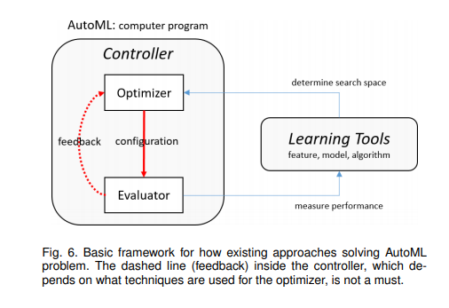
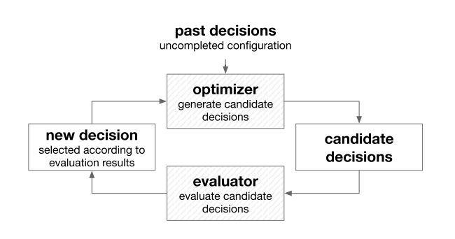
Basic framework

Proposed AutoML framework:

Evaluator: The duty of the evaluator is to measure the performance of the learning tools with configurations provided by the optimizer. After that, it generates the feedback to the optimizer

Optimizer: Update or generate the configuration for learning tools. The search space of the optimizer is defined by learning tools

Taxonomies of AutoML Approaches

Based on what and how to automate

1. ‘What to automate’: by Problem Setup

   • general case
     • Feature Engineering
     • Model selection
     • Algorithm selection
   • Deep learning
     • Neural Architecture Search

2. ‘How to automate’: by Techniques

   • Basic

     • Optimizer: Optimization & Search
       • Simple search approaches: grid search, random search
       • Optimization from samples
       • Gradient descent
       • More complex ones: reinforcement learning and automatic differentiation
     • Evaluator: Performance Evaluation
       • Basic evaluation strategies

   • Advanced

     Experienced techniques learn and accumulate knowledge from past searches or external data. They usually need to be combined with basic ones

     • Meta Learning
     • Transfer Learning

     They both try to make use of external knowledge to enhance basic ones for the optimizer and evaluator

We focus on supervised AutoML approaches in this survey as all existing works for AutoML are supervised ones

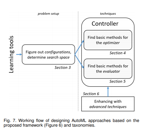
Working flow based on Taxonomies

3. Problem settings

• What learning process we want to focus on?
• What learning tools can be designed and used?
• What are resultant corresponding configurations?

By answering the questions we can define the search space for an AutoML approach

3.1 Feature Engineering

Automatically construct features from the data so that subsequent learning tools can have good performance

The above goal can be further divided into two sub-problems:

• creating features from the data
• enhance features’ discriminative ability (For now, we focus on this)

Feature Enhancing Methods

• Dimension reduction

  select a subset of features from the original ones, popular methods are greed search and lasso

  Feature projection transforms original features to a new low-dimensional space, e.g., PCA, LDA, autoencoders

• Feature generation

  construct new features from the original ones based on some pre-defined operations.

  e.g., multiplication of two features and standard normalization

• Feature encoding

  re-interprets original features based on some dictionaries learned from the data. Training samples that are not discriminable in the original space become separable in the new space.

  e.g. sparse coding, local-linear coding, kernel methods(used with SVM)

Search space

• hyper-parameters of tools, and configuration exactly refers to these hyper-parameters

  e.g., determine the dimension of features when employing PCA, and the level of sparsity if sparse coding is used

• contains features to be generated and selected, commonly considered in feature generation. Basically, the search space if spanned by operations on original features, from plus, minus and times operation

3.2 Model selection

• pick up some classifiers
• set their corresponding hyper-parameters

Classification Tools

e.g.,

• tree classifiers
• linear classifiers
• kernel machines
• deep networks

Search space

The candidate classifiers and their corresponding hyper-parameters make up the search space

3.3 Optimization Algorithm Selection

Automatically find an optimization algorithm so that efficiency and performance can be balanced

Optimization algorithms

• Gradient descent(GD), suffers from convergence and expensive per-iteration complexity.
• L-BFGS, Limited memory-BFGS, more expensive but converges faster
• SGD, stochastic gradient descent, each iteration is very cheap but many iterations are need before convergence

Search space

determined by configurations of optimization algorithms, contains the choice of optimization algorithms and the values of their hyper-parameters

3.4 Full scope

Two classes of full-scope AutoML approaches

• general case

  combination of feature engineering, model selection and algorithm selection

• NAS

  target at searching good deep network architectures that suit learning problem

  Three reasons why discuss it in parallel with the full scope

  • hot research topic
  • application domain for deep networks is relative clear
  • domain specific network architectures can fulfill the learning purpose, where feature engineering and model selection are both done by NAS

Network Architecture Search(NAS)

e.g. CNN

• number of filters
• filter height
• stride height
• filter width
• stride width
• skip connections

4. Basic techniques for optimizer

After the search space is defined, we need to find an optimizer to guide the search in the space

Three important questions:

• What kind of search space can the optimizer operate on?
• What kind of feedbacks it needs?
• How many configurations it needs to generate/update before a good one can be found? – efficiency

Divide techniques into three categories:

• simple search approaches
• optimization from samples
• gradient descent

4.1 Simple search approaches

make no assumptions about the search space

each configuration in the search space can be evaluated independently

• Grid search(brute force)

  Enumerate every possible configurations in the search space

  Discretization is necessary when the search space is continuous

• Random search

  Randomly samples configurations in the search space

  Random search can explore more on important dimensions than grid search

Simple search does not exploit the knowledge gained from the past evaluations, it is usually inefficient.

4.2 Optimization from samples

iteratively generates new configurations based on previously samples

more efficient than simple search methods

does not make specific assumptions about the objective

divide into 3 categories:

• heuristic search
• model-based derivative-free optimization
• reinforcement learning

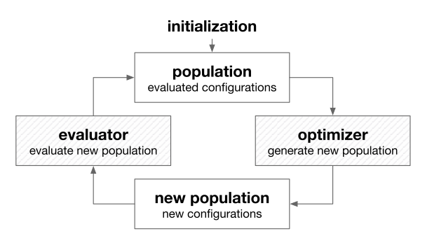
Heuristic search 启发式搜索

often inspired by biologic behaviors and phenomenon

widely used to solve optimization problems that are non-convex, non-smooth, or even non-continuous

population-based optimization methods

popular heuristic search methods:

• Popular swarm optimization(PSO) 粒子群优化

  inspired by the behavior of biological communities that exhibit both individual and social behavior

  the population is updated by moving towards the best individuals

  PSO optimizes by searching the neighborhoods of the best samples

  PSO has been used for model selection, feature selection for support vector machine (SVM), and hyper-parameter tuning for deep networks

• Evolutionary algorithms

  inspired by biological evolution

  generation step contains crossover and mutation

  • crossover 交叉

    involve two different individuals, combine them in some way to generate an new individual

  • mutation 变异

    slightly changes an individual to generate a new one

  With crossover mainly to exploit and mutation mainly to explore, the population is expected to evolve towards better performance.

  Has been applied in feature selection and generation and model selection

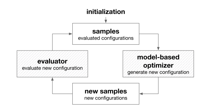
Model-based Derivative-Free Optimization

Model-based optimization builds a model based on visited samples

Full utilization of feedbacks from the evaluator helps it generate more promising new samples

Popular methods:

• Bayesian optimization

  builds a probabilistic model

  define an acquisition function based on the probabilistic model

  a new sample is generated by optimizing the acquisition function and used to update the probabilistic model once its evaluated

• classification-based optimization(CBO)

  classification-based optimization learns a classifier that divides the search space into positive and negative areas.

  Then, new samples are randomly generated in the positive area where it is more likely to get better configurations

  efficient

• Simultaneous optimistic optimization(SOO)

  branch-and-bound optimization algorithm

  tree structure is built on the search place

  SOO deeply explores the search space by expanding leaf nodes

  Through the tree model, SOO can balance exploration and exploitation to find the global optimum then the objective function is Local-Lipschitz continuous

  suffer from curse of dimensionality

Reinforcement learning

can solve problems with delayed feedbacks

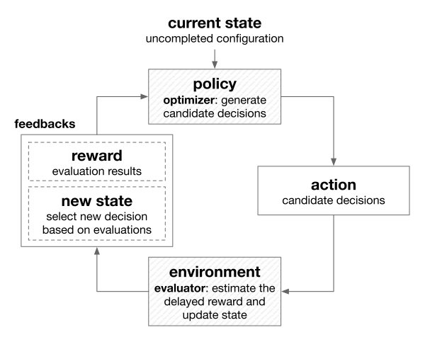
The feedbacks(reward and state) do not need to be immediately returned once an action is taken. They can be returned after performing a sequence of actions

RL is recently used in NAS. Design of one layer can be seen as one action given by the optimizer. Due to the delayed feedbacks, AutoML with reinforcement learning is highly source-consuming.

Some current endeavors addressing this problems are learning transferable architectures from smaller data sets, and cutting the search space by sharing parameter

RL has also been used for optimization algorithms search, automated feature selection and training data selection in active learning

4.3 Gradient descent

Optimization problems of AutoML is very complex, and the objective is usually not differentiable or even not continuous.

In AutoML problem, the gradients need to be numerically computed

1. This can be done with finite differentiation methods but at high costs

   The computation of exact gradients relies on the convergence of model training

   Through inexact gradient, hyper-parameters can be updated before the model training converges, which makes gradient descent method more efficient

2. Another way to compute gradients is through reversible learning (automatic differentiation)

   compute gradients with chain rule

   backpropagation process of network training

4.4 Greedy search

natural strategy to solve multi-step decision making problem

follows a heuristic that makes locally optimal decision at each step with the intent of finding a global optimum

applied in feature selection and submodular optimization

E.g., in NAS problem, greedy search is applied for multi-attribute learning problems

greedy search is also employed to search block structures within a cell, which is later used to construct a full CNN

4.5 Other techniques

popular one is to change the landscape of the search space so that more powerful optimization techniques can be used

E.g., discrete search space to continuous, then use gd instead of RL. or encoder-decoder framework

5. Basic techniques for evaluator

Very time-consuming as it involves model training for most of the times

Three important questions:

• Can the technique provide fast evaluation?
• Can the technique provide accurate evaluation?
• What feedbacks need to be provided by the evaluator?

Tradeoff between the first and second question

Lower accuracy but larger variance

5.1 Techniques

Direct evaluation

simplest method

the model parameters are learned on the training set, and the performance is measured on the validation set afterwards

accurate but expensive

Sub-sampling

training time depends heavily on the amount of training data

train parameters with a subset of the training data

either using a subset of samples, a subset of features or multi-fidelity(多高保真) evaluations

Early stop

it is usually used to cut down the training time for unpromising configurations

If a poor early-stage performance is observed, the evaluator can terminate the training and report a low performance to indicate that the candidate is unpromising

introduces noise and bias to the estimation, maybe some features eventually turn out to be good after sufficient training

Parameter reusing

use parameters of the trained models in previous evaluation

to warm-start the model training for the current evaluation

parameters learned with similar configurations can be close with each other

as different start point may lead convergence to different local optima, it sometimes brings bias in the evaluation

one of the most straightforward applications of transfer learning

Surrogate evaluator

cut down the evaluation cost is to build a model that predicts the performance of given configurations, with experience of past evaluations

serving as surrogate evaluators, sparse the computationally expensive model training, significantly accelerate AutoML

the application scope is limited to hyper-parameter optimization since other kinds of configurations are often hard to quantize, meta-learning are promising to address this problem

6. Experienced Techniques

experienced techniques that can improve the efficiency and performance of AutoML

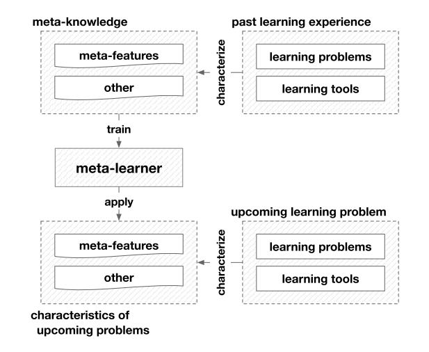
• meta-learning

  meta-knowledge about learning is extracted

  meta-learner is trained to guide learning

• transfer learning

  transferable knowledge is brought from past experiences to help upcoming learning

They all aim to exploit experience gained from past learning practices

Some researchers also take transfer learning as a special case of meta-learning

6.1 Meta-learning

Categorizing them into three general classes:

• for the evaluator
• for the optimizer
• for dynamic configuration adaptation

General Meta-Learning Framework

Configuration Evaluation

Most computation-intensive step: configuration evaluation, due to cost of model training and validation

Categorize：

• Model evaluation

  meta knowledge: meta features of learning problems and the empirical performance of different models

  meta learner: map the meta-features to the performance, applicability, ranking of models

• General configuration evaluation

  E.g., in ExploreKit, ranking classifiers are trained to candidate features

Meta-learners are trained to predict the performance or suitability of configurations

where all possible choices have been enumerated, best configurations can be directly selected according to the scores and rankings predicted by the meta-learner

Configuration Generation

Meta-Learning can also facilitate configuration generation by learning

• Promising configuration generation

  meta-knowledge indicate the empirically good configurations are extracted

  meta-learner, take learning problem as input and predict promising configurations

  it is also possible to learn promising configuration generation strategies(e.g., feature transformations)

• Warm-starting configuration generation

  better initialize configuration search

  given a new learning task, to identify the past tasks that are closest to it in the meta- feature space, and use their best-performing configurations to initialize search

• Search space refining

  make effort to evaluate the importance of configurations, or identify promising regions in the search space

Dynamic Configuration Adaptation

the data distribution varies even in a single data set, especially in data streams

concept drift: such change in data distribution

Classical ml, concept drift is often priorly assumed or posteriorly detected

Meta-learning can help to automate this procedure by detecting concept drift and dynamically adapting learning tools

• Concept drift detection

  some papers…

• Dynamic configuration adaptation

  Once the concept drift is detected, configuration adaptation can be carried out

  similar in promising configuration generation

6.2 Transfer learning

By using the knowledge from the source domain and learning task

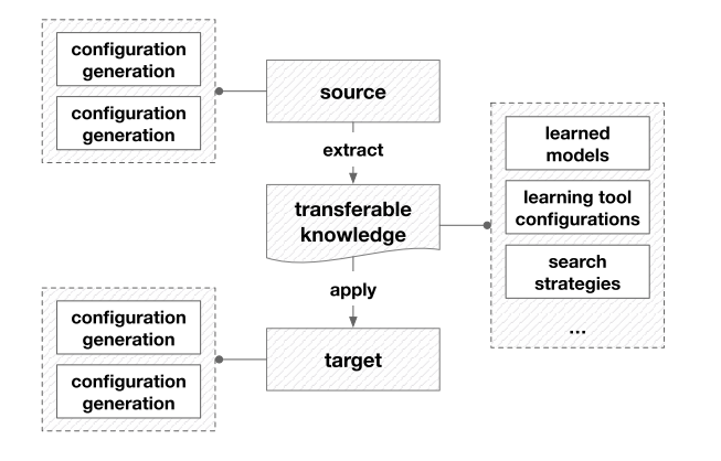
• configuration generation(for the optimizer)
• configuration evaluation(for the evaluator)

Configuration Generation

reuse trained surrogate models or promising search strategies from past AutoML search(source) and improve the efficiency in current AutoML task(target)

• surrogate model transfer

  transfer the surrogate model, or its components such as kernel function

  general case is hyper-parameter optimization machine

• network cell transfer

Multi-task learning, is also employed to help configuration generation

Configuration Evaluation

transfer knowledge from previous configuration evaluations

widely employed in NAS approaches to accelerate the evaluation of candidate architectures

• Model parameter transfer

  initialize network with transferred feature layers, followed by fine-tuning

• Function preserving transformation

  first proposed in Net2Net, where new networks are initialized to represent the same functionality of a given trained model

  also inspires new strategies to explore the network architecture space

7. Representative examples

7.1 Model selection using Auto-sklearn

CASH problem

aim to minimize the validation loss with respect to the model as well as its hyper-parameters and parameters

7.2 Reinforcement learning for NAS(NASNet)

RL

transfer learning

parameter sharing

greedy search

CNN with less depth and fewer parameters with comparable performance to that of state- of-art CNN designed by humans.

7.3 Feature Construction using ExploreKit

• candidate feature generation

• candidate feature ranking

  meta learning employed to accelerate

  with historical knowledge on feature engineering

• candidate feature evaluation and selection

8. Summary

8.1 A brief history

8.2 Current status in the academy and industry

ICML NIPS KDD AAAI IJCAI JMLR

8.3 Future works

Problem setup

automatically creating features from the data

Techniques

• Basic techniques

  higher efficiency

  simultaneously optimize configurations and parameters

• Experienced techniques

  • meta learning

    how to automate meta-learning..

  • transfer learning

    automatically determine when and how to transfer what knowledge

• Applications

  • active learning
  • neural network compression
  • semi-supervised learning

Theory

• Optimization theory

  convergence speed

• Learning theory

  which type of problems can or cannot be addressed by an AutoML approach

Clarify AutoML approach generalization ability

AdaNet